Nonlinear multi-wave coupling and resonance in elastic structures
Kovriguine DA
Solutions to the evolution equations describing the phase and amplitude modulation of nonlinear waves are physically interpreted basing on the law of energy conservation. An algorithm reducing the governing nonlinear partial differential equations to their normal form is considered. The occurrence of resonance at the expense of nonlinear multi-wave coupling is discussed.
Introduction
The principles of nonlinear multi-mode coupling were first recognized almost two century ago for various mechanical systems due to experimental and theoretical works of Faraday (1831), Melde (1859) and Lord Rayleigh (1883, 1887). Before First World War similar ideas developed in radio-telephone devices. After Second World War many novel technical applications appeared, including high-frequency electronic devices, nonlinear optics, acoustics, oceanology and plasma physics, etc. For instance, see [1] and also references therein. A nice historical sketch to this topic can be found in the review [2]. In this paper we try to trace relationships between the resonance and the dynamical stability of elastic structures.
Evolution equations
Consider a natural quasi-linear mechanical system with distributed parameters. Let motion be described by the following partial differential equations
(0)
 ,
where
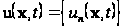 denotes
the complex
 -dimensional
vector of a solution;
 and
 are the
 linear differential operator matrices characterizing the inertia and
the stuffiness, respectively;
 is the
-dimensional
vector of a weak nonlinearity, since a parameter
 is small1;
 stands for the spatial differential operator. Any time
the sought variables of this system
are referred to the spatial Lagrangian coordinates
.
Assume that the motion is defined by the Lagrangian . Suppose that at the degenerated Lagrangian produces the linearized equations of motion. So, any linear field solution is represented as a superposition of normal harmonics:
.
Here denotes a complex vector of wave amplitudes2; are the fast rotating wave phases; stands for the complex conjugate of the preceding terms. The natural frequencies and the corresponding wave vectors are coupled by the dispersion relation . At small values of , a solution to the nonlinear equations would be formally defined as above, unless spatial and temporal variations of wave amplitudes . Physically, the spectral description in terms of new coordinates , instead of the field variables , is emphasized by the appearance of new spatio-temporal scales associated both with fast motions and slowly evolving dynamical processes.
This paper deals with the evolution dynamical processes in nonlinear mechanical Lagrangian systems. To understand clearly the nature of the governing evolution equations, we introduce the Hamiltonian function , where . Analogously, the degenerated Hamiltonian yields the linearized equations. The amplitudes of the linear field solution (interpreted as integration constants at ) should thus satisfy the following relation , where stands for the Lie-Poisson brackets with appropriate definition of the functional derivatives. In turn, at , the complex amplitudes are slowly varying functions such that . This means that
(1) and ,
where the difference can be interpreted as the free energy of the system. So that, if the scalar , then the nonlinear dynamical structure can be spontaneous one, otherwise the system requires some portion of energy to create a structure at , while represents some indifferent case.
Note that the set (1) can be formally rewritten as
(2) ,
where
is a vector function. Using the polar coordinates
 ,
eqs. (2) read the following standard form
(3)
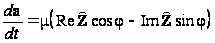 ;
 ,
where
 .
In most practical problems the vector function
 appears as a power series in
.
This allows one to apply procedures of the normal transformations and
the asymptotic methods of investigations.
Parametric approach
As an illustrative example we consider the so-called Bernoulli-Euler model governing the motion of a thin bar, according the following equations [3]:
(4)
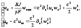
with the boundary conditions

By
scaling the sought variables:
 and
 ,
eqs. (4) are reduced to a standard form (0).
Notice
that the validity range of the model is associated with the wave
velocities that should not exceed at least the characteristic speed
 .
In the case of infinitesimal oscillations this set represents two
uncoupled linear differential equations. Let
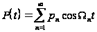 ,
then the linearized equation for longitudinal displacements possesses
a simple wave solution
 ,
where
the frequencies
 are coupled with the wave numbers
 through the dispersion relation
 .
Notice that
 .
In turn, the linearized equation for bending oscillations reads3
(5)
 .
As
one can see the right-hand term in eq. (5) contains a spatio-temporal
parameter in the form of a standing wave. Allowances for the this
wave-like parametric excitation become principal, if the typical
velocity of longitudinal waves is comparable with the group
velocities of bending waves, otherwise one can restrict
consideration, formally assuming that
 or
 ,
to the following simplest model:
(6)
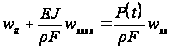 ,
which takes into account the temporal parametric excitation only.
We can look for solutions to eq. (5), using the Bubnov-Galerkin procedure:
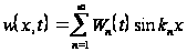 ,
where
 denote the wave numbers of bending waves;
 are the wave amplitudes defined by the ordinary differential
equations
(7)
 .
Here

stands
for a coefficient containing parameters of the wave-number detuning:
 ,
which, in turn, cannot be zeroes;
 are the cyclic frequencies of bending oscillations at
 ;
 denote the critical values of Euler forces.
Equations (7) describe the early evolution of waves at the expense of multi-mode parametric interaction. There is a key question on the correlation between phase orbits of the system (7) and the corresponding linearized subset
(8)
 ,
which
results from eqs. (7) at
.
In other words, how effective is the dynamical response of the system
(7) to the small parametric excitation?
First,
we rewrite the set (7) in the equivalent matrix form:
 ,
where
 is the vector of solution,
 denotes the
 matrix of eigenvalues,
 is the
matrix with quasi-periodic components at the basic frequencies
 .
Following a standard method of the theory of ordinary differential
equations, we look for a solution to eqs. (7) in the same form as to
eqs. (8), where the integration constants should to be interpreted as
new sought variables, for instance
 ,
where
 is the vector of the nontrivial oscillatory solution to the uniform
equations (8), characterized by the set of basic exponents
 .
By substituting the ansatz
 into eqs. (7), we obtain the first-order approximation equations in
order
 :
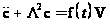 .
where
the right-hand terms are a superposition of quasi-periodic functions
at the combinational frequencies
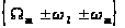 .
Thus the first-order approximation solution to eqs. (7) should be
a finite quasi-periodic function
4,
when the combinations
 ;
otherwise, the problem of small divisors
(resonances) appears.
So,
one can continue the asymptotic procedure in the non-resonant case,
i. e.
 ,
to define the higher-order correction to solution5.
In other words, the dynamical perturbations of the system are of the
same order as the parametric excitation. In the case of resonance the
solution to eqs. (7) cannot be represented as convergent series in
.
This means that the dynamical response of the system can be highly
effective even at the small parametric excitation.
In a
particular case of the external force
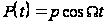 ,
eqs. (7) can be highly simplified:
(9)
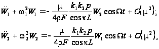
provided
a couple of bending waves, having the wave numbers
 and
 ,
produces both a small wave-number detuning
 (i. e.
 )
and a small frequency detuning
 (i. e.
 ).
Here the symbols
 denote the higher-order terms of order
 ,
since the values of
 and
 are also supposed to be small. Thus, the expressions
;
can
be interpreted as the phase matching
conditions creating a triad of waves
consisting of the primary high-frequency longitudinal wave, directly
excited by the external force
 ,
and the two secondary low-frequency bending waves parametrically
excited by the standing longitudinal wave.
Notice that in the limiting model (6) the corresponding set of amplitude equations is reduced just to the single pendulum-type equation frequently used in many applications:

It
is known that this equation can possess unstable solutions at small
values of
 and
 .
Solutions to eqs. (7) can be found using iterative methods of slowly varying phases and amplitudes:
(10)
 ;
 ,
where
 and
 are new unknown coordinates.
By substituting this into eqs. (9), we obtain the first-order approximation equations
(11)
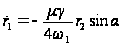 ;
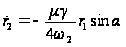 ,
where
 is the coefficient of the parametric excitation;
 is the generalized phase governed by the following differential
equation
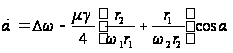 .
Equations (10) and (11), being of a Hamiltonian structure, possess the two evident first integrals
 and
 ,
which
allows one to integrate the system analytically. At
 ,
there exist quasi-harmonic stationary solutions to eqs. (10), (11),
as
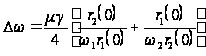 ,
which forms the boundaries in the space of system parameters within the first zone of the parametric instability.
From the physical viewpoint, one can see that the parametric excitation of bending waves appears as a degenerated case of nonlinear wave interactions. It means that the study of resonant properties in nonlinear elastic systems is of primary importance to understand the nature of dynamical instability, even considering free nonlinear oscillations.
Normal forms
The linear subset of eqs. (0) describes a superposition of harmonic waves characterized by the dispersion relation
 ,
where
 refer the
branches of the natural frequencies depending upon wave vectors
 .
The spectrum of the wave vectors and the eigenfrequencies can be