Planning of mobile complete set for a rural wind generator
The axial flux permanent magnet topology should also be looked into to compare it to the radial flux type.
The exact costs of assembling and maintaining the recycled wind turbine should also be incorporated in the design procedure.
With the little output power generated in this thesis, this project must definitely be taken further to alleviate the electricity problems in South Africa.
References
Socio-economic rights project, “The right to affordable electricity” copyright @ community law centre 2002
IDASA, idasa.za
Department of Minerals and Energy, White Paper on the Renewable Energy Policy of the Republic of South Africa. August 2002
Department of Minerals and Energy, White Paper on the Renewable Energy Policy of the Republic of South Africa. November 2003
Sathyajith Mathew, “Wind Energy-Fundamentals, Resource Analysis and Economics ” © Springer- Verlag Berlin Heidelberg 2006
Smail Khennas, Simon Dunnett and Hugh Piggott, “Small wind systems for rural energy services”. ITDG Publishing 2003
Kevin Reeves, “The design and Implementation of a 6kW wind turbine simulator” University Of Cape Town, South Africa, Oct 2004
FrequentlyAskedQuestions magnetsales/Design/FAQs_frames/FAQs_2.htm © 2000 Magnet Sales & Manufacturing Company, Inc
R.C. Bansal, T.S. Bhatti, D.P. Kothari, “On some of the design aspect of wind energy conversion systems” Birla Institute of technology and science, Pilani, September 2002
Jacek F. Gieras, Mitchell Wing, “Permanent magnet motor technology-Design and Applications” 1st edition. Marcei Dekker, Inc. 1997
Prof E. J. Odendal, “Design, construction and testing of a small wind generator with electronic controller for domestic use”. University of Natal, Durban
Jacek F. Gieras, Mitchell Wing, “Permanent magnet motor technology-Design and Applications” 2nd edition. Marcei Dekker, Inc. 1997
P.C. Sen, “Principles of electric machines and power electronics” 2nd edition. John Wiley & Sons
Bhag S. Guru, Huseyin R. Hiziroglu, “Electric Machinery and Transformers” 3rd edition. Oxford University Press, Inc. 2001
Dr. James Livingston, “Magnetic Materials Overview”
E. Muljadi, C.P. Butterfield, Yih-Huei Wan, “Axial flux, Modulator, Permanent-Magnet with a Toroidal winding for wind turbine applications”. Cole Boulevard, Nov 1998
Magfag, 2003 by Force Field
M.A. Khan, P. Pillay, “Design of a PM wind generator, optimised for energy capture over a wide operating range”
Joe Naylor, “Speakers with Alnico magnets vs. speakers with ceramic magnets”
Hybrid (Wind/Solar/LP Gas) Systems for Rural Community Development, “Electrifying South Africa for prosperity and development”. Upper Maphaphethe by Mike Wintherden
Danish Wind Industry Association, ‘Guided Tour’ online htt://windpower/en/tour/wres/betz.htm
Lysen, E.H., ‘Introduction to Wind Energy’ CWD,2nd edition, p.p 51-73
Ripinga Nonkululeko, “Comparison of grid and off-grid rural electrification, based on the actual installation in Limpopo Province”. University of Cape Town, Oct. 2005
Alfred Still & Charles S. Siskind, “Elements of electrical machine design”. 3rd edition. McGraw-Hill Book company,inc. 1954
Appendix A
Graphs of output rms induced voltage and flux of the generator
1. Commercial Standard Magnets
Ceramic FLux_RMS = 0.0175
EMF_RMS = 3.6075
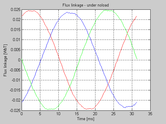
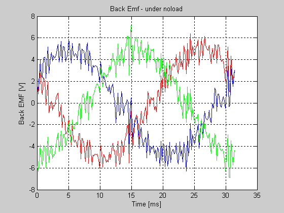
Alnico FLux_RMS =0.0168
EMF_RMS = 5.1619
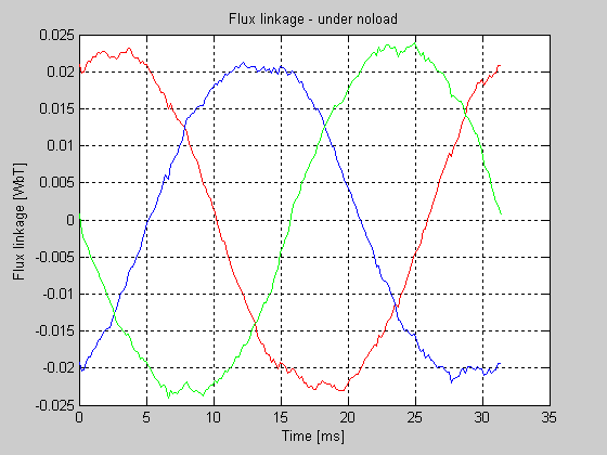
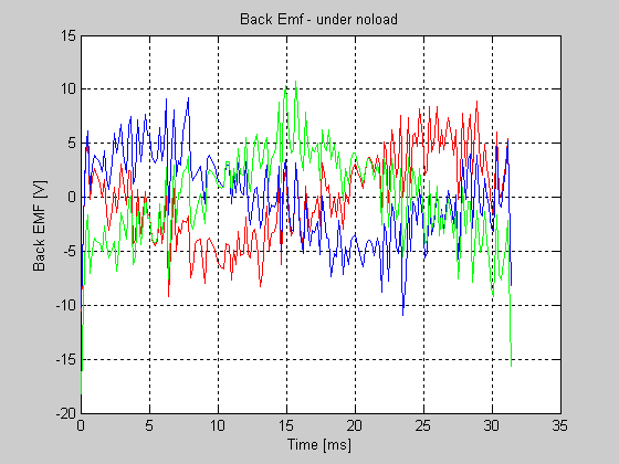
NdFeB FLux_RMS = 0.0459
EMF_RMS = 9.4262
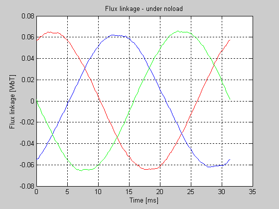
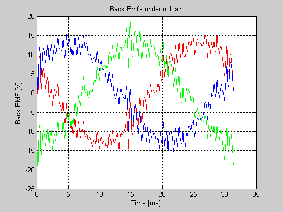
2. Loud Speaker Magnet
FLux_RMS = 0.0171
EMF_RMS = 3.4987
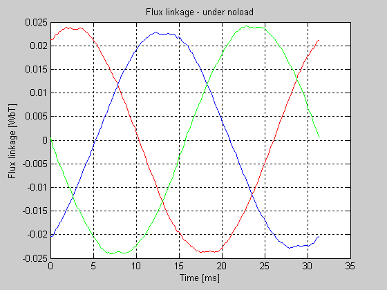
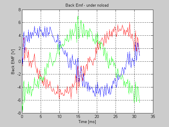
Appendix B
Matlab code for sketching the output emf and flux of the generators
% EMF calculation from FEMM
%By Maribini Manyage
clc
clear all; close all;
P = 2;
w = 1912; %mechanical speed in rpm
freq = (w*pi/30)*P/(4*pi); %frequency
XA = load('flux_link_A.txt');
XB = load('flux_link_B.txt');
XC = load('flux_link_C.txt');
beta = XA(:,1); % angle between Is_r and d-axis [elec degrees]
alpha = beta - beta(1,1); % Rotor position in [elec degrees] from Zero
time = alpha*(pi/180)/(2*pi*freq);%*1000; %time
flux_link_A = 2*XA(:,2);
flux_link_B = 2*XB(:,2);
flux_link_C = 2*XC(:,2);
% Perform spline in order to differentiate flux linkage vs time
pp_flux_A = spline(time,flux_link_A);
pp_flux_B = spline(time,flux_link_B);
pp_flux_C = spline(time,flux_link_C);
% extracting piecewise polynomial coefficients and derivation
[hgt,wdth] = size(pp_flux_A.coefs);
clear AA;
for k = 1:hgt
AA(k,:) = polyder(pp_flux_A.coefs(k,:));
end
dpp_flux_A = MKPP(time,AA)
[hgt,wdth] = size(pp_flux_B.coefs);
clear AA;
for k = 1:hgt
AA(k,:) = polyder(pp_flux_B.coefs(k,:));
end
dpp_flux_B = MKPP(time,AA);
[hgt,wdth] = size(pp_flux_C.coefs);
clear AA;
for k = 1:hgt
AA(k,:) = polyder(pp_flux_C.coefs(k,:));
end
dpp_flux_C = MKPP(time,AA);
%back emf
emf_A = ppval(time,dpp_flux_A);
emf_B = ppval(time,dpp_flux_B);
emf_C = ppval(time,dpp_flux_C);
figure(1);
plot(time*1000,flux_link_A,'r-');
hold on;
plot(time*1000, flux_link_B,'b-');
plot(time*1000, flux_link_C,'g-');
title('Flux linkage - under noload');
xlabel('Time [ms]'),ylabel('Flux linkage [WbT]')
grid;
figure(2);
plot(time*1000,emf_A,'r-');
hold on;
plot(time*1000, emf_B,'b-');
plot(time*1000, emf_C,'g-');
title('Back Emf - under noload');
xlabel('Time [ms]'),ylabel('Back EMF [V]')
grid;
x = length(flux_link_A);
FLux_RMS = norm(flux_link_A)/sqrt(x)
y = length(emf_A);
EMF_RMS = norm(emf_A)/sqrt(y)