Interpolation, approximation and differential equations solvers
The following methods were described in this semester:
Rectangular method
Trapezoidal rule
Simpson's rule
Gauss-Legendre method
Gauss-Chebyshev method
2.2.1 Rectangular method
The most straightforward way to approximate the area
under a curve is to divide up the interval along the x-axis between
 and
 into a number of smaller intervals, each of the same length. For
example, if we divide the interval into
 subintervals, then the width of each one will be given by:

The approximate area under the curve is then simply the sum of the areas of all the rectangles formed by our subintervals:

The summary approximation error for
intervals with width
 is less than or equal to
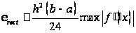
Thus it is impossible to calculate maximum of the derivative function, we can estimate integration error like value:

2.2.2 Trapezoidal rule
Trapezoidal rule is a way to approximately calculate the
definite integral. The trapezium rule works by approximating the
region under the graph of the function
 by a trapezium and calculating its area. It follows that
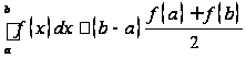
To calculate this integral more accurately, one first
splits the interval of integration
 into n smaller subintervals, and then applies the trapezium rule on
each of them. One obtains the composite trapezium rule:

The summary approximation error for
intervals with width
is less than or equal to:

2.2.3 Simpson's rule
Simpson's rule is a method for numerical integration, the numerical approximation of definite integrals. Specifically, it is the following approximation:

If the interval of integration
is in some sense "small", then Simpson's rule will provide
an adequate approximation to the exact integral. By small, what we
really mean is that the function being integrated is relatively
smooth over the interval
.
For such a function, a smooth quadratic interpolant like the one used
in Simpson's rule will give good results.
However, it is often the case that the function we are
trying to integrate is not smooth over the interval. Typically, this
means that either the function is highly oscillatory, or it lacks
derivatives at certain points. In these cases, Simpson's rule may
give very poor results. One common way of handling this problem is by
breaking up the interval
into a number of small subintervals. Simpson's rule is then applied
to each subinterval, with the results being summed to produce an
approximation for the integral over the entire interval. This sort of
approach is termed the composite Simpson's rule.
Suppose that the interval
is split up in
subintervals, with n an even number. Then, the composite Simpson's
rule is given by

The error committed by the composite Simpson's rule is bounded (in absolute value) by

2.2.4 Gauss-Legendre method and Gauss-Chebyshev method
Since function values are given in fixed points then
just two points Gauss-Legendre method can be applied. If
 is continuous on
 ,
then

The Gauss-Legendre rule
 G2(
f ) has degree of precision
 .
If
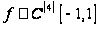 ,
then
 ,
where
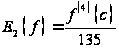
It should be noted that even in case of two points
method we have to calculate values of the function in related to
 ,
 ,
this values could be evaluated by linear interpolation (because it is
necessary to avoid oscillations), so estimation of integration error
become very complicated process, but this error will be less or equal
to trapezoidal rule.
Mechanism of Gauss-Chebyshev method is almost the same like described above, and integration error will be almost the same, so there is no reason to use such methods for the current problem.
Problem 3
3.1 Problem definition
It is well known that the third order Runge-Kutta method is of the following form
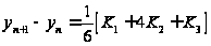 ,
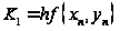


Suppose that you are asked to derived a new third order Runge-Kutta method in the following from
,


Find determine the unknowns
 ,
 ,
 and
 so that your scheme is a third order Runge-Kutta method.
3.2 Problem solution
Generally Runge-Kutta method looks like:
 ,
where coefficients
 could be calculated by the scheme:


The error function:

Coefficients
 ,
 ,
 must be found to satisfy conditions
 ,
consequently we can suppose that for each order of Runge-Kutta scheme
those coefficients are determined uniquely, it means that there are
no two different third order schemes with different coefficients. Now
it is necessary to prove statement.
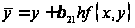
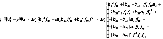
For
 ,
 :

 ;
 ;

 ;
 ;






 ;

 ;
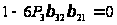 ;
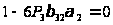
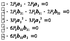
Thus we have system of equations:
Some of coefficients are already predefined:
 ;
 ;
 ;
 ;
 ;
 ;
 ;



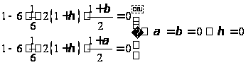

Obtained results show that Runge-Kutta scheme for every order is unique.
Problem 4
4.1 Problem definition
Discuss the stability problem of solving the ordinary
equation
 ,
 via the Euler explicit scheme
 ,
say
 .
If
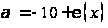 ,
how to apply your stability restriction?
4.2 Problem solution
The Euler method is 1st order accurate. Given scheme could be rewritten in form of:
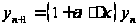
If
 has a magnitude greater than one then
 will tend to grow with increasing
 and may eventually dominate over the required solution. Hence the
Euler method is stable only if
 or:
